Link back to Home page

Link to typed notes

1. Into to Stats

Mean

Median: the middle value in an ordered list of observations
Model the most frequent value in the data

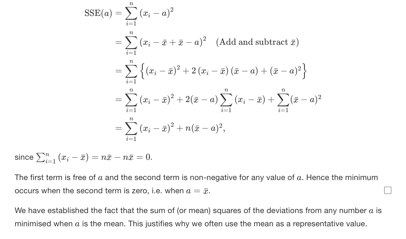
SSE = sum of squares of errors

SAE = sum of absolute errors

Theorem: $\overline{x}$ minimizes the SSE

Theorem: median minimizes the SAE

The main idea is to look at slopes.. and then just find the value where the gradient changes from negative to positive

Proof is long and convoluted, link to it here, at some point it will make sense, until then, link here

Measures of spread

IQR = Interquartile range, difference between $Q_1$ and $Q_3$

The variance is:

Notice how the $SSE(a)=\sum _{i=1}^n(x_i-a{)}^2$

And we found SSE is minimized at $a=\overline{x}$

So

To calculate the mean, we just divide by the the total population: $n-1$
There is a reason we do $n-1$, it gives us an unbiased estimate of the sample variance - this is covered later in the course

Proof of variance (not examined by still good for understanding)

However, there is a more useful form of the variance, the proof of which is given below:

Then we split the sum:

As the $2\overline{x}$ is a constant, we can factor that out of the sum

Now using the definition of the mean:

So to rearrange

Therefore:

The standard deviation is the square root of variance

2. Intro to Probability

Definitions

Definition Random experiment: one in which we do not know exactly what the outcome of the experiment will give.
Definition Sample space - the set of all possible outcomes. Denoted by capital $S$
Definition Event - particular result of the random experiment, a subset of the sample space. Denoted by capital letters

Everything that is random is denoted by a capital letters. Lowercase is where we have observed

Definition Union - $A\cup B$ - either $A$ or $B$ occurs or both occur
Definition Intersect - $A\cap B$ - both $A$ and $B$ must occur

Definition Mutually exclusive - $A\cap D=\mathrm{\varnothing }$ - A and D have no outcomes in, i.e. cannot happen at the same time

Definition Complement - $A^{‘}$ - all of the outcomes not in A. Note the things below:

The statement above basically means that everything in A and not A is the sample space

Axioms of probability

$P\{A\cup B\}=P\{A\}+P\{B\}$ provided that $A$ and $B$ are mutually exclusive

Combinatorics

The entire point of this section is fairly simple: being able to count outcomes without listing them all

There are two main questions that will determine which formula we have to use.

1. Does the order matter? If it does, then we use permutations, otherwise combinations
2. Do we replace items after choosing? If yes, with we use the with replacement cases

Permutations

The scenario here is that we have $n$ distinct items and we want to arrange them $k$ of them in a specific order.

Think of it like filling $k$ positions on a shelf:

• The first sport can take $n$ choices
• The second spot can take $n-1$ choices since the first one is already used
• The third can take $n-2$ choices and so on...

So the total number of ordered arrangements (aka permutations) is:

Multiply numerator and denominator by $(n-k)!$ then we get the simplified definition below

Combinations

Now suppose we want to choose $k$ items from $n$ distinct ones, but the order doesn't matter.

In other ways, when we go from permutations to combinations, we don't care what order the items are chose in, only which items were chosen. So as we've already counted the same group multiple times for every possible order with permutations, we need to divide by how many times we've 'overcounted', which is $k!$

Conditional probability and Bayes’ Theorem

At its simplest, probability is just chance of an event, so it's:

Conditional probability is the probability event $A$ happening given that another event $B$ has already happening.
The formal definition is given below:

When we arrange, we can get:

Bayes’ Theorem

Now, when we know something about one conditional event, but want to know about the reverse, we can use Bayes' Theorem:

We can derive the numerator by just substituting $A\cap B$ from the rearrangement above.

Bayes' Theorem is used widely when in medical test scenarios as it allows people to update their belief about an event after new evidence appears. To think about using an analogy:

• We start with a prior belief $P(B)$
• Get new evidence $P(A)$
• And then we update our belief to $P(A|B)$

Independence

Intuitively, events $A$ and $B$ are independent if occurrence of one event does not affect the probability that other event occurs.

Knowing that one event happened gives you no new information about the other.

Notice how this is different to mutually exclusive, which means that both events cannot happen at the same time, so $P(A\cap B)=0$

Formally,
If

Then

Proof of Independence of complementary events

If $A$ and $B$ are independent, so are $A^{‘}$ and $B^{‘}$

We want to show the following below:

And how using using the general addition rule, we can rewrite the above as

Given that $A$ and $B$ are independent, we can make the substitution

This can be factorise as:

Which simplifies to $P(A^{‘})P(B^{‘})$

3. Probability Distributions

Random variables are denoted by uppercase letters, like $X,Y,Z$

A random variable is just a mapping from the outcomes space to the real line, so the combined probability of all values of a random variable is 1

Discrete Random Variable (DRV)

Definition
DRV - discrete random variable. If a random variable has a finite value

A DRV takes specific values, like heads in coin flips and we can count how many outcomes there are. We assign probabilities to each value individually:

And so to find the total probability up to some value $k$, we just need to sum the DRVs:

For a DRV, we define a function $$ f(x) = P(X=x) $$
The function $f(x)$ is just the probability mass (pmf) or the probability function. As the total probability must be 1 and all probabilities must be non-negative, we need:

• $f(x)\ge 0\mathrm{\forall }x$
• $\sum _{\mathrm{\forall }x}f(x)=1$

Continuous Random Variable (CRV)

Definition
CRV - Continous random variable. When a variable can take any value on the real line

There are infinitely many possible values, so the probability of hitting any exact number, $P(X=x)=0$

So instead, we can talk about densities, the probability per unit of $x$

Probability Density Function (PDF)

This function essentially tells us how densely probability is packed around each value.
This is defined as:

That's why for CRVs, integration replaces summation, it's the continuous version of adding up infinitely small pieces.

For the pdf, we need:

• $f(x)\ge 0\mathrm{\forall }x$
• ${\int }_{-\mathrm{\infty }}^{\mathrm{\infty }}f(x)dx=1$

Cumulative distribution function (CDF)

This function calculates the probability of the random variables up to its arguments:

For a DRV, it's defined as:

And for a CRV, the CDF is defined as:

So the CDF is essentially the area under the PDF curve up to $x$

Relationship between PDF and CDF

For a CRV, the PDF is the derivative of the CDF

If

And we differentiate both sides with respect to $x$ we get:

What this tells us that the PDF is just the slope of the CDF. Where the CDF rises, the PDF is large, lots of probability density there. And where the CDF is flat, the PDF is small.

Expectation

Think of expectation (or the expected value) as the long-run average value of a random variable if you repeated the experiment infinitely many times.

For example, if you roll a fair rice, the values are in the set of $[1,6]$
Each roll has probability $1/6$.
Then

You'll never roll a $3.5$, but if you roll hundreds of times, you average approaches $3.5$

Formal definition

For a DRV with possible values $x_1,x_2...x_n$, and probabilities $p_i=P(X=x_i)$:

And for CRV with PDF $f(x)$:

Same idea, we're just replacing the sum with an integral because now the variable takes infinitely many values

Expectation of a uniform distribution function

Say we have $X\sim U(a,b)$, a uniform distribution where each probability is equally likely anywhere between $a$ and $b$

The PDF is:

Then the expectation is:

Which is just the midpoint of the interval

Expectation of a function

If you have some function of the random variable say $Y=g(X)$, then it's expectation is

• Discrete:

• Continuous:

This is extremely useful as it lets us find things like:

• $E[X^2]$ which is later needed for variance
• $E[\sin x]$
• etc.

Linearity of expectation

this is probably one of the most useful properties in probability.
For any random variable $X$, $Y$, and constants $a,b$:

The reason we can do this is because expectation acts like a weighted average. If we stretch all our data by a factor of $a$, then the average stretches by $a$, and then if we shift all the data by $b$, the average shifts by $b$.

Proof of linearity

For a DRV:

But since $Y=aX+b$, we can rewrite the above expression as:

And now we can distribute the sum:

The first part of the sum is just $aE[X]$ by definition of expectation, and the second part is $b(1)$ since the probabilities sum to $1$.
So we have:

For a CRV:

And again, as $Y=aX+b$, we can write it as:

The first part is again just $aE[X]$ by definition and the second part equals $1$ since the total probability is $1$.

Note on notation here: capital $X$ represents the random variable, i.e the function that maps outcomes to numbers. And an $x$ represents a value that $X$ might take. So when we're computing the expectation of $E[Y]$, we're summing or integrating over all the possible values it can take, so we replace $X$ with $x$.

Expectation of symmetric random variable

A random variable $X$ is called symmetric about a point $c$ if its PDF (or PMF) satisfied:

If $X$ is symmetric about $c$, then $E(X)=c$

Intuitively, think of this as the centre of mass of the function. If the PDF or PMF is symmetric about a point $c$, then for every value to the left of $c$, there's an equal value to the right of $c$ with the same probability. This property saves us from having to do nasty integrals when finding expectations.

Proof for symmetric random variable

First, let $Y=X-c$. This means that $Y$ is symmetric about $0$, so our PDF satisfies the following property of an even function:

Then we have:

We can substitute $z=-y$ and flip the integral limits to get:

As as $f(-z)=f(z)$

Variance

We already saw that the expectation $E(X)$ is the long run average of $X$. Now, if we want to do know how spread out the values are from the mean, we can use the variance.

If we wanted to measure how far (deviated) each possible value of $X$ is from the mean, that's $X-E(X)$. But if we took lots of samples from the population, we could average those deviations. But the positive and negatives ones cancel, so we instead square them to get the magnitude:

For very large $n$, we know that $\overline{x}\approx E(X)$, as for a large enough sample, the sample mean gets closer to the actual mean. So if we write $\mu =E(X)$, the sample variance is:

So when $n$ is large, this will be close to :

This variance is therefore defined by:

Proving variance

There is a more useful form of variance, which we can prove from the definition below:

After expanding the bracket

Take the expectation of both sides:

Using the linearity of expectation, we can split and pull constants out to get:

After simplifying we have:

Linearity of variance

If $Y=aX+b$, then

• Scaling by $a$ stretches or shrinks the spread
• Adding $b$ shifts everything, so no change in spread

To prove this, we can use the definition of variance and some algebra

After substituting in for $E(Y)$ using the linearity of expectation we have:

We can do some cancelling of the $b$ to get:

As $(X-E(X){)}^2=Var(X)$ by definition, we have:

Sample median of random variables

Quantiles

For any $0<p<1$, the $p$-quantile $q$ solves $F(q)=p$. So if $F$ is invertible, then $q=F^{-1}(p)$

Standard Discrete Distributions

Bernoulli Distributions

Bernoulli trails are a name for a set of independent trials, where each trial has only two possible outcomes- success, and failure.

For a Bernoulli trial:

$X\sim$ Bernoulli($p$)

The Bernoulli distributions has pmf:

For this distribution, the expectation is:

And the variance is:

Binomial distribution

Defined as:

If $X$ is the number of successes ($S$) out of $n$ Bernoulli trials

PMF for the Binomial

To find the PMF, we want to find $f(x)=P(X=x)$, i.e. the probability of $x$ Successes, and $(n-x)$ Failures

The probability of the outcomes can be given by:

So to generalize,
The pmf is:

Now one might wonder how we know that $$ \sum_{x=0}^{n}f(x) = 1$$
… by using the binomial theorem

Now if we choose $a=p$ and $b=(1-p)$, then

Expectation and Variance of a Binomial function

Intuitively, think of $X$ (the total number of successes) as being made up on $n$ smaller random variables, one for each trial

Let

Where $X_i$ is $1$ if the trial is a success and $0$ if the trial is a failure. So each $X_i$ is a Bernoulli random variable with parameter $p$

Now, we know that for a single trial, the expectation of a Bernoulli variable is

And since each expectation is linear, the expectation of the sum is

Where each $E(X_i)=p$

So we get that expectation of a binomial is

The variance is

The proof of this is left as an exercise to the reader

Geometric Distribution

Intuitively, the geometric distribution is the first one that captures the "keep trying until you succeed" idea. So imagine we're running an experiment where:

• Each trial is independent
• Each trial has a probability of success $p$
• We keep repeating until we get our first success

The random variable $X$ represents the trial number on which the first success occurs.

PMF for a geometric distribution

To get a success on the $x$-th trial, we must have $(x-1)$ failures first, followed by $1$ success. Each success has a probability of $p$ and each failure has a probability of $(1-p)$

CDF

Note - R assumes the number of failures until first success, instead of the number of trials until the first success. So if $X\sim Geo(p),X-1$ is the number of failures

Memoryless distribution

The geometric distribution is memoryless, i.e

This means just that the probability we still have to wait for $s$ for more trials doesn't depend on how long we've already waited for. No other discrete distribution has this property!

Expectation of a geometric distribution

For the intuition, imagine playing a game where:

• Every trial has a chance $p$ of success

How many tries do we expect to need before success?

If $p$ was large, then we'd succeed quickly, resulting in a small expected $X$
If $p$ was small, then we would have to wait much longer, so a large expected $X$

So the average should:

• Decrease when $p$ increases
• Increase when $p$ decreases

The proof involves using negative binomial series, something which will not be covered in lectures, but it’s in the notes. A much nicer proof is covered in 2nd year Statistical Inference module

Variance of a geometric distribution

Going back our previous analogy, the variance here is how spread out the time between our successes. So if $p$ was big, we would succeed quickly, resulting in a smaller variance. And if $p$ was small, we could have to wait a long time, so a big variance

Hypergeometric Distribution

This distribution is all about sampling without replacement, i.e. the realistic binomial

Suppose we have a population of $N$ total individuals:

• A proportion $p$ are of type $S$ (success)
• The remaining $1-p$ are of type $F$ (failures)

So the total number of type $S$ individuals is $Np$ and type $F$ is $N(1-p)$

Now, we want to sample $n$ individuals without replacement. Let $X$ = the number of type $S$ Is our sample, then $X$ follows a hypergeometric distribution:

Then it's PMF is given by:

The numerator counts how many ways to get exactly $x$ succeses, and $n-x$ failures, and the denominator normalises so that the probabilities sum to 1

Expectation

Notice how the expectation is the same as the binomial distribution, and that's because we are drawing without replacement

Variance

Negative Binomial Distribution

The negative binomial distribution models the number of trials needed to achieve a fixed number of successes, $r$ in independent Bernoulli trials. In other words, it's how long till we get $r$ successes.

If we just wanted $1$ success, then the negative binomial is the same as the geometric distribution, which stop when we get our first success.

PMF

Imagine flipping a coin where $p=0.3$ of getting heads. And we want to know how many flips it will takes to get 3 heads. That random variable $X$ follows a negative binomial distribution, the PMF for which is given by:

Expectation

Each success takes $1/p$ trials on average, and we need $r$ of them

Variance

Poisson Distribution

The Poisson distribution models the number of times an event happens in a fixed interval. It includes things like the number of emails you might get per hour, we can't predict exactly when then event happens, but over many intervals, the average rate stays the same.

So formally, It's the limit as $n\to \mathrm{\infty }$ and $p\to 0$ of $Bin(n,p)$ so that $\lambda =np$ is fixed. And we can often use the Poisson as an approximation to binomial when

• $n$ is large
• $p$ is small and
• $np=\lambda$ is moderate

PMF

The PMF of this function can be derived by taking the limit of the binomial where we want to rearrange this and substitute for $p=\lambda /n$

Variance

If events occur randomly and independently, then the variability of counts around the means grows proportionally to the mean. So, the mean = variance in this case

Therefore, the expectation and variance are the same for the Poisson distribution

Uniform Distribution

PDF - as this is a continuous distribution

Expectation

Variance

Exponential Distribution

This distribution is bit like a continuous version of the geometric distribution, and it connects really nicely with the Poisson process. The exponential models the waiting time until the next event in a Poisson process. So if:

• events occur randomly and independently in time
• At a constant average rate $\lambda$ (events per unit time)
  Then the waiting time $X$ between two successive events is:

So the Poisson counts how many events occur in a fixed time interval, whereas the exponential measures how long between events

PDF

The full proof involves the gamma function, which is given is the official lecture notes

Expectation

If events occur at $\theta$ per unit time, the average wait, intuitively, is $\frac{1}{\theta }$ time units

Variance

This one isn't immediately obvious, but the spread of waiting time grows as $\theta$ grows

CDF

The cdf for $x>0$ is defined as:

Quantiles

As talked about earlier, quantiles tells us how far along the probability distribution we have to go to capture a certain proportion of data. So for a CRV $X$ with CDF $F(X)$, the $p$-th quantile is the value $q$ s.t.:

So we're solving for the $x$ value that corresponds to the cumulative probability $p$. And to find theat value, we need the inverse of the CDF, i.e. $q=F^{-1}(p)$

For the exponential distribution, recall that the cdf is $F(x)=1-e^{-\theta x}$, so to solve for $q$, we have:

And that's our quantile function

Memorylessness (Again!)

The exponential distribution is also memoryless, as it’s just a continuous version of the geometric.

So the probability that we want to wait at least $t$ more time units, given that we've already waited $s$ time units without an event, is the same as if we just started waiting now. i.e. past waiting doesn't change future expectation

Normal Distribution

PDF

The CDF is just

3b1b has some good videos on this

To show that sum of all probabilities is $1$, we use the property of the Gamma function;

And the standard normal $Z=\frac{x-\mu }{\sigma }$. The full proof can be found in the notes

Expectation

Variance

Linear Transformation

We can also standardise any normal to get

Probabilities using tables

Given the standard normal distribution with $Z$, we can use one universal table for all the normal distribution as the standard normal is just a shift and stretch of every normal curve

So if we want probability for $P(a\le X\le b)$, we can use the standard normal to get:

And then we ca use the normal CDF $\varphi (z)=P(Z\le z)$ to get the probability

Log-Normal Distributions

If $X\sim N(\mu ,{\sigma }^2)$, then the random variable $Y=\exp (X)$ is the log-normal random variable

Expectation

Variance

#finishexplaination

Joint Distributions

Up to now, we've mostly dealt with one random variable at a time, eg: $X$ = height of a person. But in the real world, we often want to study two random variables together, eg:
$X$ = height
$Y$ = weight
And we want to know how these two relate, and that's essentially what joint distributions are about

So when we have two random variables, $X$ and $Y$, instead of having probabilites of single values of $X$, we have probabilities of pairs of values ($x,y$)

Discrete Case

IF $X$ and $Y$ are discrete (like dice rolls, counts), then the joint PMF is:

This would like a table of probabilities, one for each combination of $x$ and $y$, and all probabilities must be

• non negative
• sum to $1$ across all $x,y$

Continuous case

If $X$ and $Y$ are continuous, then the joint PDF is $f(x,y)$ s.t.

The method above uses bivariate integration, which is just the same as finding the volume under a curve if we think about integration as finding the are under a curve.

Marginal Distributions

Each random variable has its own individual distribution, even when considered together. And these are called marginal distributions. This is because we get them by summing or integrating the joint distributions along the margins.

Discrete

This basically means to get the probability of $X$, add up all the probabilities for each possible $y$

Continuous

Expectation of $g(X,Y)$

Now consider we want to find the average (expected) value of something that depends on both $X$ and $Y$, so we have a generalised formula for expectation

This is the same as the single-variable version, but now in two dimension

Covariance

Covariance tells us how two random variables move together

The intuition behind this is essentially:

• If $X$ and $Y$ increase together - then covariance is positive
• If one goes when the other goes down, it's negative
• If they move independently, then covariance is around $0$

Correlation - normalised covariance

Correlation then, is just the scaled version of covariance so its unit free and lies between $-1$ and $1$ and it’s given by:

• If the correlation is $+1$, then there is a positive linear relationship
• If it's $-1$, then it's a negative linear relationship
• If its $0$, then there is no linear relationship

I can’t be bothered enough to do a proof for this, so yeah.

So correlation just shows how strong and in which direction $X$ and $Y$ move

In function terms two random variable are independent if knowing one tells us nothing about the other:

So if $X$ and $Y$ are independent $⟹$ they have $0$ correlation, but the converse is not true

Sums of Random Variables

Independent Binomial Random Variables

If $X\sim B(m,p)$ and $Y\sim B(n,p)$, then

The proof is in notes, but otherwise this makes intuitive sense.

IF $Y=X_1+X_2+\dots X_n$ with $E(X_i)={\mu }_i$ and $Var(X_i)={\sigma }_i^2$

Then:

This is actually a pretty neat way to derive the expectation and variance for the Binomial and the negative binomial distribution:

Central Limit Theorem